MATH ILLUSTRATIONS

QUICKLY CREATE ACCURATE DRAWINGS FOR TEST and PRESENTATIONS

Introducing Math Illustrations, an easy intuitive way to create geometric diagrams for documents and presentations.

By combining the constraint-based architecture of Geometry Expressions with easy-to-use drawing and graphing features, Math Illustrations lets you create more effective geometry figures for your students in less time.

Draw Quickly:Quickly create drawings by using a constraint-based model. With a single click, add leader lines and dimension arrows to specify lengths, angles, distances and radii.

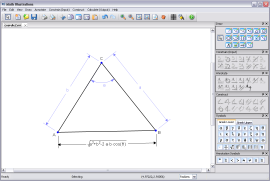
When you create a diagram in Math Illustrations you get all the symbols without any effort! When you constrain or annotate a line, the length symbols is added automatically. This is true for any annotation or constraint that you add!The Power of Constraints Plus the Flexibility of AnnotationsWhen you draw with constraints you don't have to worry about lining up shapes so they appear to have a certain relationship. If you want a line tangent to a circle, simply constrain it to be. You are then free to move or resize your circle and the line will automatically remain tangent to the circle!When you want to label an angle, length, etc without constraining its value use can use annotations. An annotation label can be anything you want -- including a mix of text and 2D math.

DRAW QUICKY

Draw Accurately:

You can set the lengths of lines, value of angles, and size of radii in your figures. If side A of a triangle is length 4 and side B is length 6, you can be sure that side B is 1.5 times longer than side A.

Drawing to Scale

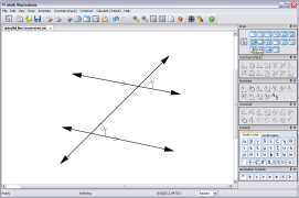
With the help of constraints, drawing figures to scale happens automatically. If line AB is constrained to a distance of 4 and line CD to a distance of 8, CD will automatically be twice as long as AB.

The same is true of angles. If you want a triangle with angles 30°, 60° and 90° simply constrain two of them (the software will figure out the third).

Of course you may want to purposefully draw a figure that is not to scale. This is where the annotations come in. Using annotations instead of constraint you can set a distance or angle to be anything you want!

DRAW ACCURATELY

Export Easily:

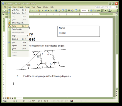
Draw a selection around your figure to place it on the clipboard in raster and vector format. Paste this directly into Word, PowerPoint, Photoshop, iWork -- you name it! We also support file export of EPS, EMF, PNG, JPG, Tiff and more.

Export to your document in 3 easy steps

Exporting to Word, PowerPoint, iWork, Paint, Photoshop, Fireworks is extremely easy in Math Illustrations. By drawing a selection box around your image both a vector graphic image and raster image is placed on your clipboard. When you paste into another program the vector image will be pasted if it is supported, otherwise the raster image will be pasted.

Here is a quick run down of the steps needed:

How to...draw a pantograph with Math Illustrations

A Pantograph is a mechanism which creates a half or double scaled version of whatever you trace.

Here is how to model it in Geometry Expressions:

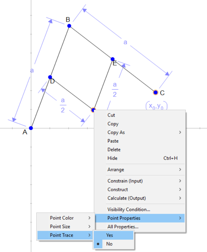Draw lines AB, BC with A at the origin.
Create D,E, the midpoints of AB and BC.
Draw lines DF and FE.
Constrain AB and BC to be lengtha.
Constrain DF and EF to be lengtha/2.
Constrain the coordinates of C to be (x0,y0).
In the Variables Panel, lock variable a.
Now select C and F and from the right click menu do Point Properties / Point Trace / Yes

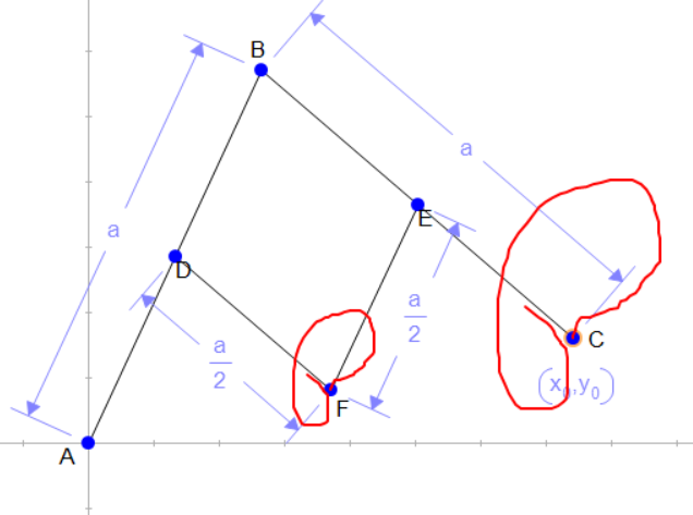Now you can drag C and you will see the trace left by both C and F

Point Traces are available in Math Illustrations v. 3.1 (and Geometry Expressions 3.3 and Mechanical Expressions 1.1).

Here is an app generated by Geometry Expressions.

Problem of the Month

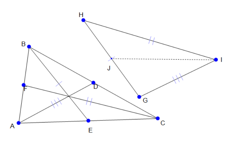Given a triangle ABC, let its medians be AD, BE and CF.

Construct a new triangle GHI whose sides have the lengths of the medians of the original triangle.

Let IJ be a median of GHI.

What is the relationship between the length of the median IJ and the lengths of the sides of the original triangle ABC?

An app which lets you explore this is here.

A Solution to June's Problem

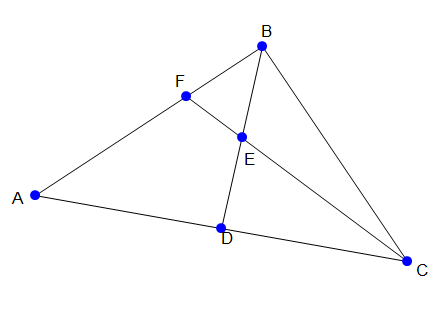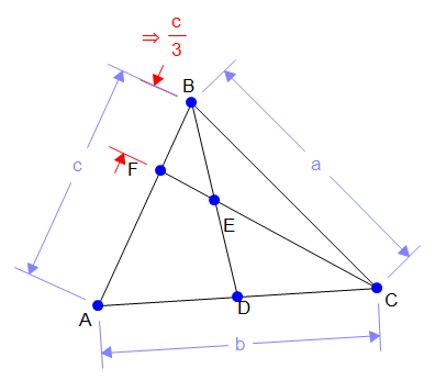
Show that the line joining the midpoint of a median to a vertex of the triangle trisects the side opposite the vertex considered.

In the diagram, D is the midpoint of AC, E is the midpoint of BD.

You are asked to show that BF is 1/3 of AB.

An app which lets you explore this ishere.

Using Geometry Expressions this is an easy result to establish.

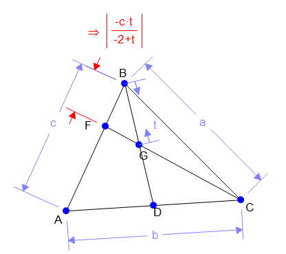
Just constrain the triangle by its side lengths, create midpoint D, then midpoint E, draw CF and constrain E to lie on it. Now measure the symbolic distance BF.

You can generalize the result by putting E at proportion t along the line BD.

Got Clock Apps? If you need some time, we're sending our geometrical Clock Apps made with Geometry Expressions to keep you entertained and up to the minute! Just click the blue image captions to try out the apps, and you can download them to put on your personal webpage. (These Clocks, with their explanatory apps are not only free of charge, but also advert free!) If you own a copy of Geometry Expressions, you can also download the .gx file to see how they are made and modify them to your preference.

To make your own personalized Clocks or other apps, get your copy of Geometry Expressions.

Clocks Volume 01 The Morphing Clock

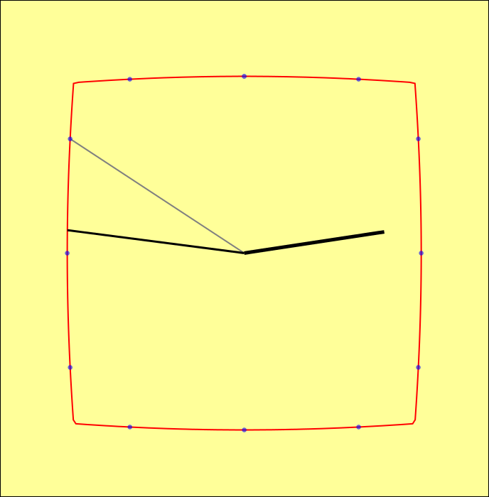
Is this clock a circle, or a square, or something in-between, or something beyond?

Morphing Clock

Not only do the hands move in this clock, but its shape changes with time. At the hour it is circular, at the quarter hours it is square and at the half hour, it has gone beyond square to a concave curved square shape. The morphing is achieved by taking a linear combination of the parametric representation of a square and a circle.


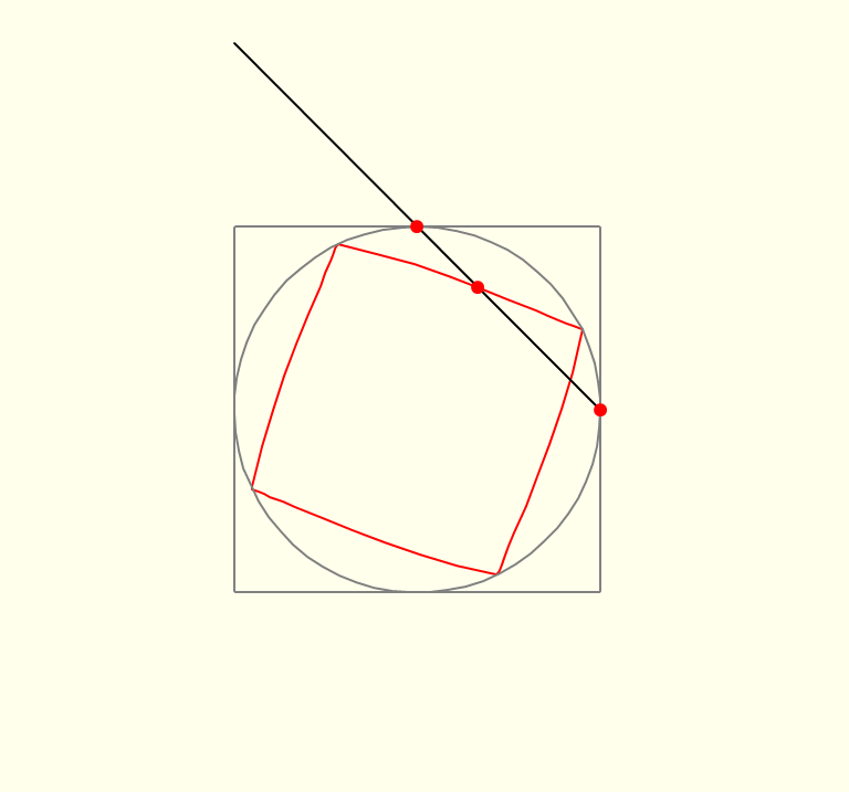
Figure 1.1 Morphing between a circle and a square

Geometrically, the morph curve is constructed

by joining two corresponding

points on the original curves by a line, and

then positioning a third point at a specific

proportion along this line (Figure 1.1).

In the figure, let parameter t specify the location of the points on the original curves (the red dots on the circle and the square), and parameter s specify the location of the morph curve's deﬁning point (the middle red dot) on the line joining the two original points.

Algebraically, if a(t) is the location of the point on the circle, and b(t) is the location of the point on the square, then the morph curve is deﬁned by:

c(t) = s.b(t)+(1-s).a(t)

If s="0," then c(t)=a(t) and the morph curve is the circle. If s="1," then c(t)=b(t) and the

morph curve is a square. If s is between 0 and 1, the morph curve is an intermediate

form.

If s goes beyond 1, the morph curve is still defined, but now we are in a sense subtracting

the circle from the square and instead of blunting the square's edges, we are exaggerating them.


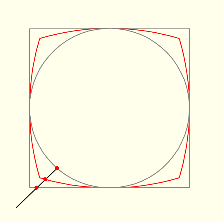
	Figure 1.2 The shape of the morph curve depends on the parametrization of the circle

The form of the morph curve depends on how the original curves are parameterized. Changing the parameterization of the original curves does not change their appearance when displayed, but it does change the appearance of the morph curve. Figure 1.2 illustrates this.


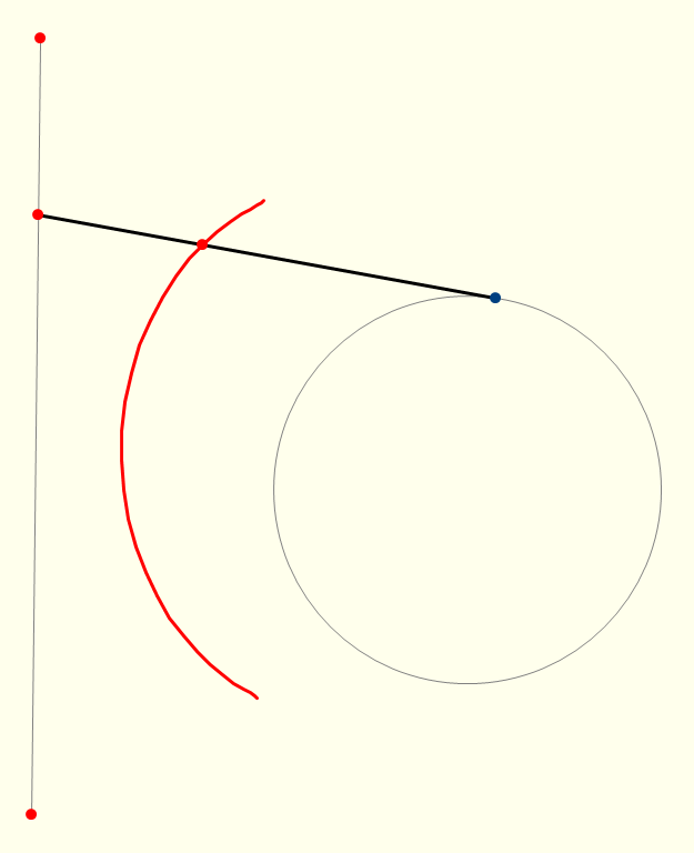
Figure 1.3 A circle morphs into a line: drag the red points on the diagram

A similar morphing operation can be defined between any pair of parametric curves, open or closed. In Figure 1.3, this is illustrated by morphing a circle into a line segment. Notice that the need to open up the circle clearly illustrates the start and end points of its parametrization. Moving the location of the destination line segment relative to the start of the circle's parametrization yields different morph curves. For example, try dragging the ends of the line segment so it is positioned to the right rather than to the left of the circle.

Another experiment to try is to drag the

end points of the line so that it is upside down.